Introduction

Raytracing is an advanced and computing-intensive method of generating graphics. Unlike traditional methods of generating objects in 3D space, this method can yield much more accurate and realistic results with the caviat of extremely high processing requirement. While the type of raytracing we have made is only suitable for still objects due to rendering times, some versions of ray tracing or pseudo raytracing exist that can be used for realtime simulations.

Initial Construction

We can start from the basics. Raytracing, in short, is the method of casting rays at each individual pixel on a ‘screen’ in front of a scene of objects in the hopes of it hitting an object. If it does, it retrieves the ‘data’ of the point of the object it hit and using that prints out a specific color on the screen. This is done for every single pixel present on screen. The result is therefore extremely accurate but incredibly time-wasting.

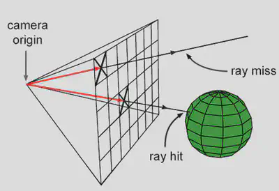
This is a simple enough strategy to start off with. The complexity comes in the data required for the color of each pixel. The first issue is to detect whether a ray is actually hitting an object. This problem is solved using standard matrix geometrical calculations based on the normal of a triangle, which most objects are made out of. Of course, customized algorithms for different types of solids can be made similarly.

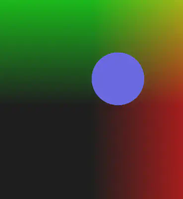
Now this process becomes extremely intensive very quickly and will take too long per frame to render, so a way out of this predicament is to split the work into multiple threads. A compute shader can accomplish This but dividing up and workspace into multiple work groups based on your graphics card and work on each one in seperate threads. This speeds up the process exponentially and eases up the work done by the CPU in calculations. A compute shader is fairly simple to set up, and for the purposes of OpenGL, we make a quad texture that covers the entire window onto which a texture is rendered and the compute shader draws pixels onto the texture mentioned.

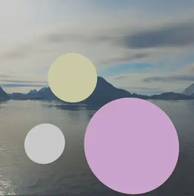
Now this looks pretty ugly without a background, so we added a skybox. It is a bounding box around a scene that appears to the viewer as the sky and background. Essentially, it is an arbitrarily large cube containing a warped texture or image to simulate atmosphere. We found this one off the internet:

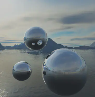
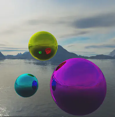
Another task we can undertake in light bouncing. We can set up ‘mirror’ objects that almost purely reflect light and iteratively create origin and destination rays from one surface to another to mimic reflection. The pixel color intensity is continuously modified by each bounce by a certain value until a ‘bounce limit’ is reached. We can reach some impressive results with this alone. You can now see behind the camera as well. We gave the spheres a slight tint:

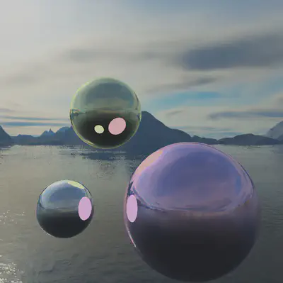
This image was generated only by reflecting each camera ray once and finding the object at that location. That’s why you see the spheres inside the reflections in solid color. Increase that limit, and you can see reflections inside reflections, and so on:

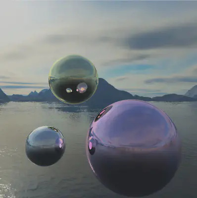
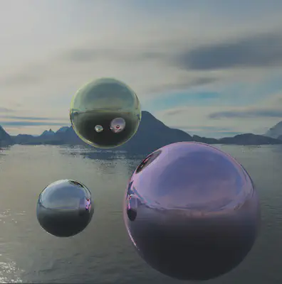
Phororealistic Rendering

Now, we can process some basic lighting, which can be as simple as checking for light bouncing off an object. If we were to process every light ray emitted from a light source and check for objects it hit it would be too much even for a compute shader to process, so a workaround is to process light in the opposite direction, i.e from the camera eye to the light source. By checking the angle between a light ray and the ray we use to trace objects we can achieve some sort of primitive lighting.

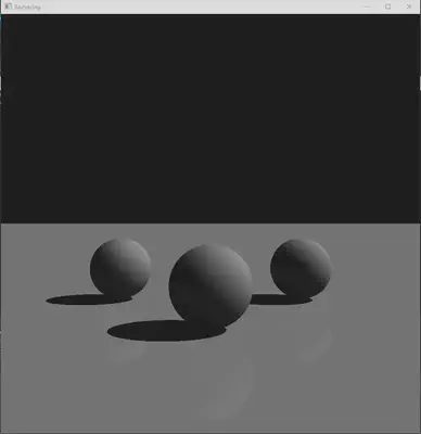
Now we are prepared to start applying James T Kajiya’s rendering equation to get better results for not just mirrors but all kinds of surfaces:

The left hand side of the equation denotes the light coming out of a point x, and is eventually what we want. The first term on RHS is the light emitted. This would be 0 for most objects, non zero for light sources. The integral describes the light that the point accumulates from the surroundings.
The integral is applied over the hemisphere around the point in question, in every direction. The first function right after the integral is the bidirectional reflectance distribution function, BRDF. This function takes as input an incoming direction and an outgoing direction and spits out a value that correlates the two. For example, for a perfect mirror, the BRDF will produce 0 for every (incoming, outgoing) pair except the ones that have their angle of reflection equal to angle of incidence. Other surfaces will have a more complicated correlation.

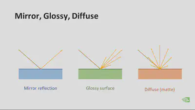
Note that “incoming” in BRDF terminology is represented as outgoing rays in the diagram because this is ray tracing, i.e., tracing the ray backwards. What actually happens in nature is that all those “outgoing” rays in the diagram come to the surface, merge into the “incoming” ray (the dark one) and hit our eye.

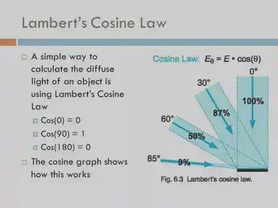
The term that comes right after it is the Lambert term which represents the Lambert cosine law.

Finally, the last term is, well, the light coming from a given incoming direction. However will we calculate this? Simple, just apply the same rendering equation at that point… and the point from there, and so on. You might start to see why this would be a problem. This is infinitely recursive and there is no way to expect a simulation to actually run this. So we have to make some compromises. One, we have to pick only a few rays to shoot out, not an infinite number of them. Second, we need a max reflections limit to prevent a ray from reflecting infinitely. Here is a very naive approach to realizing this solution:

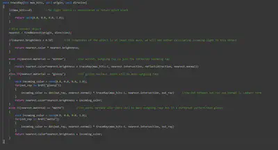
It uses recursion and a ray stops reflecting when it encounters a light source. There are two issues with this: One, GLSL (The OpenGL Shading Language) doesn’t support recursion (We can still manage to do it by using stacks but it’s going to be messy and too mentally taxing) and two, it’s going to take a very long time to render even if it did. We have to find a better solution.
Fortunately, people have already faced this issue before and have come up with elegant solutions

We can apply Monte Carlo Integration to the integral

It now reduces to a simple iterative fraction addition. This can be easily achieved using Blending methods in OpenGl and varying the alpha (transparency) value of each pixel after each frame of iteration. Then, instead of exactly calculating every single pixel value of each farme exactly, we can instead use randomized distribution as our main crutch. One single frame using randomized values would look horrible, but an accumulated iteration of slowly dimishing samples will drag the image into an eventually photorealistic image because we are increasing the N frame by frame. It will again be quite time intensive to reach enough frames to see good results, but much less than the theoretical requirement.
Next, we have to define a BRDF.

The first term represents diffuse reflection and the second, specular reflection. kd is the albedo of the surface and ks is the specular. (They control the strengths of these types of reflections). In the case of specular reflection, we also have wr and alpha. wr is just the perfectly reflected ray, and alpha works like this:

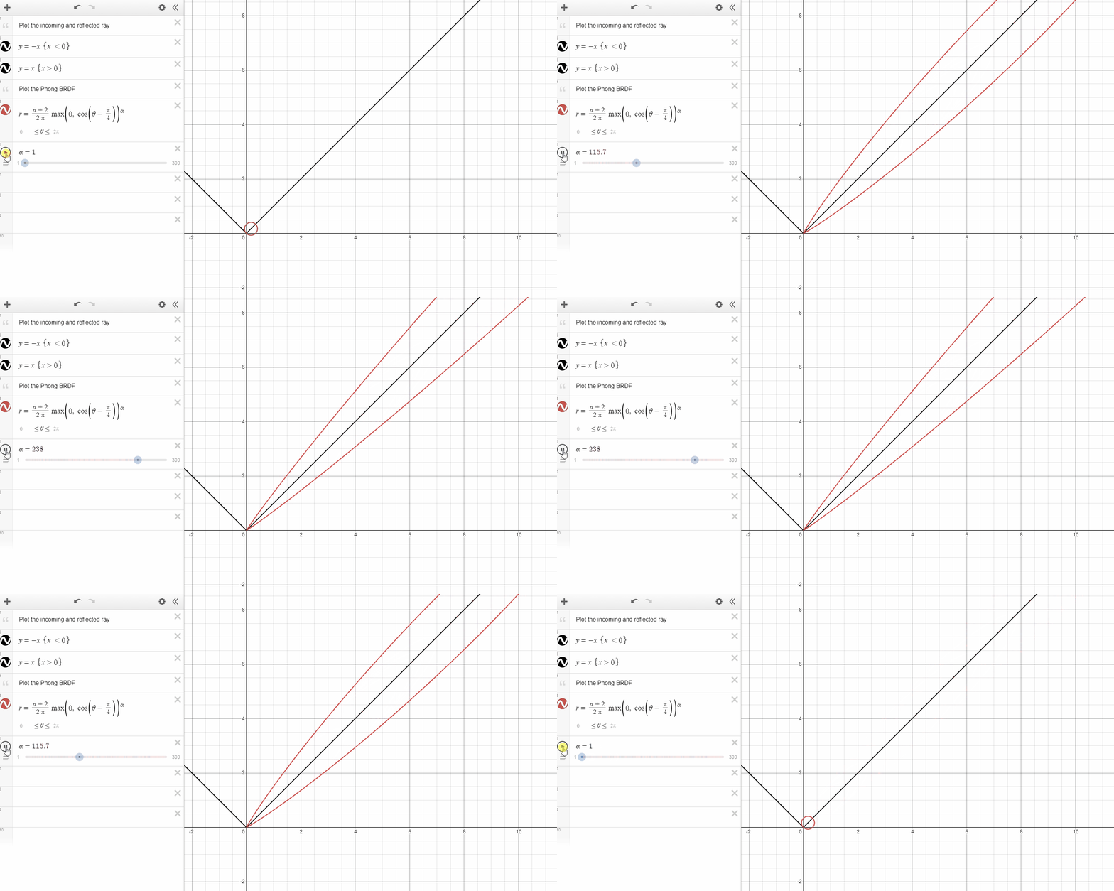
As you can see, it controls the spread of the specular (mirror-like) reflection

Piecing things together

Now that we have our code, it’s time to see what it can do

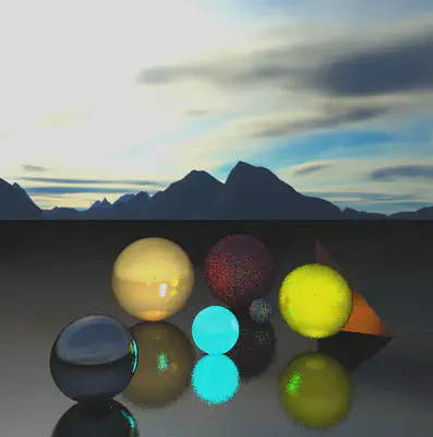
Well, the first frame looks horrible, as expected. If we let it run for a while and let the Monte Carlo summation do its magic, we get:

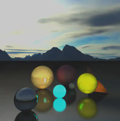
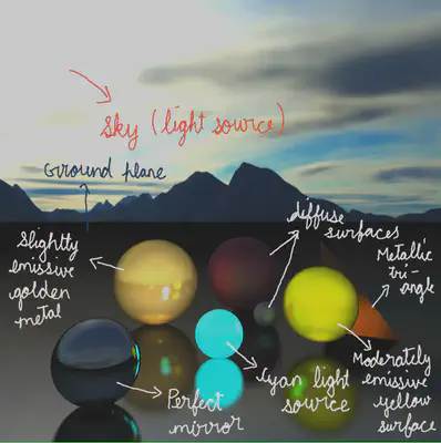
Sick. Let’s break down the scene:

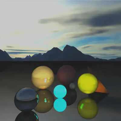
If we make the ground a perfect mirror, (set alpha very high):

If we make the ground non reflective:

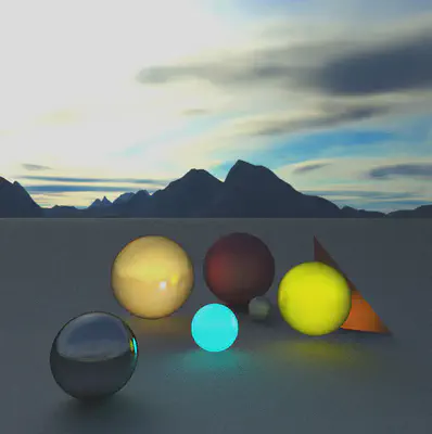
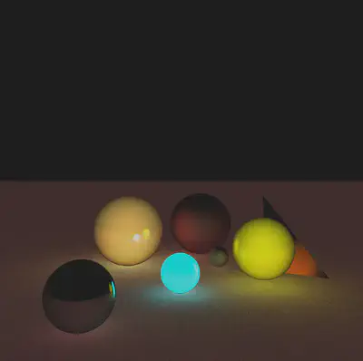
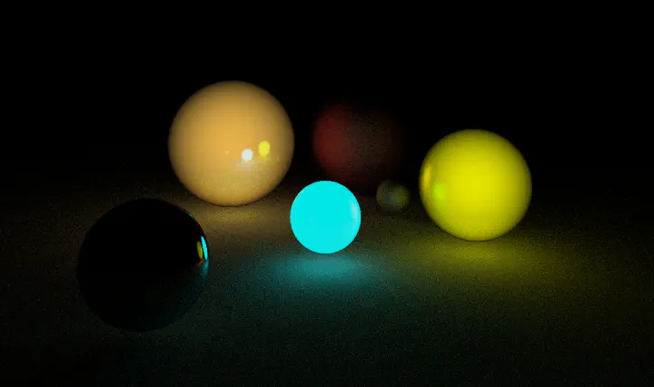
Right now, the skybox is acting as a light source with a non-zero emission value. If we make that 0, we get to see the smaller light sources in action:

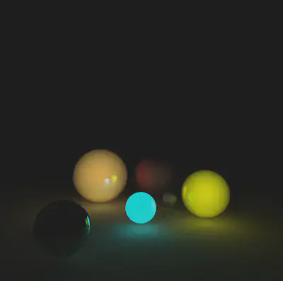
We can even make the ground emissive: